Regression

The regression helpers turn a fitted statsmodels model into tidy polars tables — the analog of R moderndive’s get_regression_table() / get_regression_points() / get_regression_summaries().

Fit models with statsmodels’ formula API, then tidy them:

import statsmodels.formula.api as smf
import moderndive as md
from moderndive import (
    get_regression_table, get_regression_points, get_regression_summaries, get_correlation,
)

houses = md.load_saratoga_houses()
model = smf.ols("price ~ living_area + bedrooms", data=houses.to_pandas()).fit()

Coefficient table (with confidence intervals)

get_regression_table(model)

shape: (3, 7)

term	estimate	std_error	statistic	p_value	lower_ci	upper_ci
str	f64	f64	f64	f64	f64	f64
"intercept"	20986.094	6816.251	3.079	0.002	7611.128	34361.06
"living_area"	93.842	3.109	30.183	0.0	87.741	99.943
"bedrooms"	-7483.095	2783.531	-2.688	0.007	-12944.988	-2021.203

Change the confidence level with conf_level= (e.g. 0.99).

Fitted values & residuals

get_regression_points(model).head()
# columns: ID, price, living_area, bedrooms, price_hat, residual

shape: (5, 6)

ID	price	living_area	bedrooms	price_hat	residual
i64	i64	i64	i64	f64	f64
1	142212	1982	3	184531.942	-42319.942
2	134865	1676	3	155816.245	-20951.245
3	118007	1694	3	157505.404	-39498.404
4	138297	1800	2	174935.767	-36638.767
5	129470	2088	3	194479.21	-65009.21

Model-fit summaries

get_regression_summaries(model)
# r_squared, adj_r_squared, mse, rmse, sigma, statistic (F), p_value, df, nobs

shape: (1, 9)

r_squared	adj_r_squared	mse	rmse	sigma	statistic	p_value	df	nobs
f64	f64	f64	f64	f64	f64	f64	i64	i64
0.578	0.578	2.5071e9	50071.187	50142.395	723.229	0.0	2	1057

Correlation

get_correlation(houses, "price ~ living_area")   # ≈ 0.759
# or: get_correlation(houses, x="living_area", y="price")

shape: (1, 1)

cor
f64
0.758674

Visualizing models

Two ports of R moderndive’s ggplot helpers, both dual-engine:

from moderndive import gg_parallel_slopes, gg_categorical_model

evals = md.load_evals()

# Parallel-slopes model: one common slope, a separate intercept per group
gg_parallel_slopes(evals, response="score", explanatory="age", by="gender")            # plotly
gg_parallel_slopes(evals, response="score", explanatory="age", by="gender",
                   engine="plotnine")

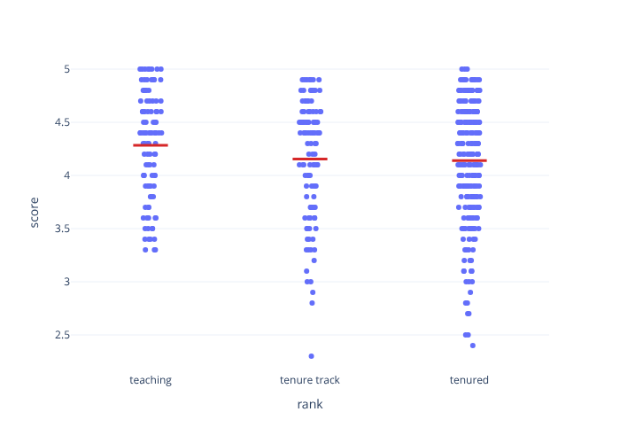
# Regression with a single categorical predictor
gg_categorical_model(evals, response="score", explanatory="rank")

For the plotnine engine you can also drop the parallel-slopes lines onto your own ggplot with geom_parallel_slopes().

Inference for regression coefficients

fit() runs the regression on every bootstrap/permutation replicate, giving a distribution per coefficient. Pair it with visualize_fit and per-facet shading:

from moderndive import specify
from moderndive.infer.viz import visualize_fit
from moderndive import shade_confidence_interval, shade_p_value

f = "price ~ living_area + bedrooms"
obs_fit = houses.specify(formula=f).fit()

# Bootstrap distribution of each coefficient → per-term CIs
boot_fit = houses.specify(formula=f).generate(reps=1000, type="bootstrap", seed=1).fit()
boot_fit.get_confidence_interval(level=0.95)          # one row per term
visualize_fit(boot_fit) + shade_confidence_interval(boot_fit.get_confidence_interval())

# Null distribution → per-term p-values, each facet shaded at its own estimate
null_fit = (
    houses.specify(formula=f).hypothesize(null="independence")
    .generate(reps=1000, type="permute", seed=1).fit()
)
null_fit.get_p_value(obs_stat=obs_fit, direction="two-sided")
visualize_fit(null_fit) + shade_p_value(obs_stat=obs_fit, direction="two-sided")

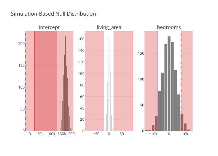
Per-facet shading works in both engines: shade_p_value / shade_confidence_interval accept the observed FitResult or a term-keyed table, and each facet is shaded from its own value.