Hypothesis testing¶

Hypothesis tests follow the same grammar as confidence intervals, with an added hypothesize() step that defines the null world, and generate() that simulates from it.

Two groups: a permutation test¶

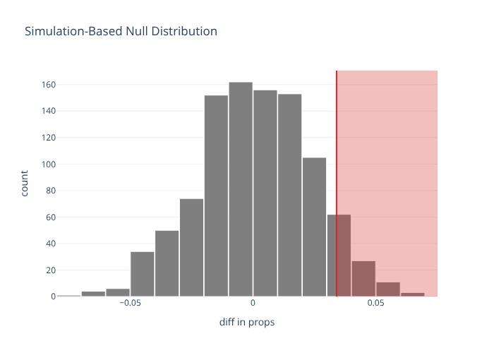
Are tracks more likely to be popular in metal than in deep house? Compare the two genres’ “popular” rates, then permute the genre labels to build the null.

import moderndive as md
from moderndive import specify, observe, get_p_value, visualize, shade_p_value

spotify = md.load_spotify_metal_deephouse()

# Observed difference in "popular" proportions, metal − deep-house
obs = observe(
    spotify, formula="popular_or_not ~ track_genre", success="popular",
    stat="diff in props", order=("metal", "deep-house"),
)

# Null: genre is independent of popularity → permute the labels
null = (
    spotify.specify(formula="popular_or_not ~ track_genre", success="popular")
    .hypothesize(null="independence")
    .generate(reps=1000, type="permute", seed=76)
    .calculate(stat="diff in props", order=("metal", "deep-house"))
)

get_p_value(null, obs_stat=obs, direction="right")

shape: (1, 1)

p_value
f64
0.075

Shade the p-value¶

visualize(null) + shade_p_value(obs_stat=obs, direction="right")

../_images/740bf8671170f1b5361f3ad35be67c52f9ce7c9f19b3daff3e4152648e08beb7.png

direction is one of "right"/"greater", "left"/"less", or "two-sided". The two-sided shading mirrors the observed statistic about 0.

One mean / one proportion (point null)¶

Use a "point" null with bootstrap resampling, supplying the hypothesized value:

age = md.load_age_at_marriage()

obs_t = observe(age, response="age", stat="t", null="point", mu=23)

null_t = (
    age.specify(response="age")
    .hypothesize(null="point", mu=23)
    .generate(reps=1000, type="bootstrap", seed=1)
    .calculate(stat="t")
)
get_p_value(null_t, obs_stat=obs_t, direction="two-sided")

shape: (1, 1)

p_value
f64
0.0

For a one-proportion test you can also simulate draws directly:

import polars as pl

coins = pl.DataFrame({"flip": ["heads"] * 30 + ["tails"] * 70})

null_p = (
    coins.specify(response="flip", success="heads")
    .hypothesize(null="point", p=0.5)
    .generate(reps=1000, type="draw", seed=1)   # "simulate" is an alias
    .calculate(stat="prop")
)

Available statistics¶

calculate(stat=...) supports the full infer vocabulary: "mean", "median", "sum", "sd", "prop", "count", "diff in means", "diff in medians", "diff in props", "ratio of means", "ratio of props", "odds ratio", "slope", "correlation", "t", "z", "F", "Chisq".

Custom test statistics¶

Beyond those strings, stat= accepts any function that takes the response (and explanatory) arrays and returns a single number — so you can infer about a statistic that isn’t built in. Here we bootstrap the interquartile range of almond weights and read off a 95% interval:

import numpy as np
from moderndive import get_confidence_interval

def iqr(response, explanatory):
    return float(np.percentile(response, 75) - np.percentile(response, 25))

boot_iqr = (
    md.load_almonds_sample_100()
    .specify(response="weight")
    .generate(reps=1000, type="bootstrap", seed=1)
    .calculate(stat=iqr)
)
get_confidence_interval(boot_iqr, level=0.95, type="percentile")

shape: (1, 2)

lower_ci	upper_ci
f64	f64
0.4	0.625

The function receives (response, explanatory) as numpy arrays (explanatory is None for a single-variable specify), and must return a scalar.