Getting started
This page walks through a complete analysis end to end, then points you at the task guides for more depth.
Install
pip install moderndive
moderndive returns polars DataFrames, but every function also
accepts pandas DataFrames as input.
Load a dataset
All datasets ship with the package and load with load_<name>():
import moderndive as md

yawn = md.load_mythbusters_yawn()
yawn.head()
| subj | group | yawn |
|---|---|---|
| i64 | str | str |
| 1 | "seed" | "yes" |
| 2 | "control" | "yes" |
| 3 | "seed" | "no" |
| 4 | "seed" | "yes" |
| 5 | "seed" | "no" |
List everything that’s available with md.available_datasets() (58 datasets), and
see Datasets for a thematic tour.
A first summary
tidy_summary gives a per-variable five-number summary (numeric) or counts
(categorical):
from moderndive import tidy_summary

tidy_summary(md.load_almonds_sample_100(), columns=["weight"])
| column | n | group | type | min | Q1 | mean | median | Q3 | max | sd |
|---|---|---|---|---|---|---|---|---|---|---|
| str | i64 | str | str | f64 | f64 | f64 | f64 | f64 | f64 | f64 |
| "weight" | 100 | null | "numeric" | 2.9 | 3.4 | 3.682 | 3.7 | 3.9 | 4.5 | 0.362 |
count_missing reports how many null values each column has, sorted worst-first
— handy for a quick data-quality check:
from moderndive import count_missing

count_missing(md.load_evals())
| column | n_missing |
|---|---|
| str | i64 |
| "ID" | 0 |
| "prof_ID" | 0 |
| "score" | 0 |
| "age" | 0 |
| "bty_avg" | 0 |
| … | … |
| "pic_outfit" | 0 |
| "pic_color" | 0 |
| "cls_did_eval" | 0 |
| "cls_students" | 0 |
| "cls_level" | 0 |
The inference pipeline
The core grammar mirrors R infer. You build a pipeline and read it like a
sentence:
from moderndive import specify, observe, get_p_value

# 1. The observed statistic: do "seeded" people yawn more than the control group?
obs = observe(
    yawn, formula="yawn ~ group", success="yes",
    stat="diff in props", order=("seed", "control"),
)

# 2. A null distribution: specify → hypothesize → generate → calculate
null = (
    yawn.specify(formula="yawn ~ group", success="yes")
    .hypothesize(null="independence")
    .generate(reps=1000, type="permute", seed=42)
    .calculate(stat="diff in props", order=("seed", "control"))
)

# 3. Summarize
get_p_value(null, obs_stat=obs, direction="right")
| p_value |
|---|
| f64 |
| 0.512 |
Each verb has a focused guide: Sampling, Bootstrapping & confidence intervals, and Hypothesis testing.
Visualizing — choose your engine
Plots default to plotly (interactive). Pass engine="plotnine" for
grammar-of-graphics output. The composition syntax is identical:
Note
The plots shown in this documentation are static images. Running the code yourself yields interactive plotly figures by default.
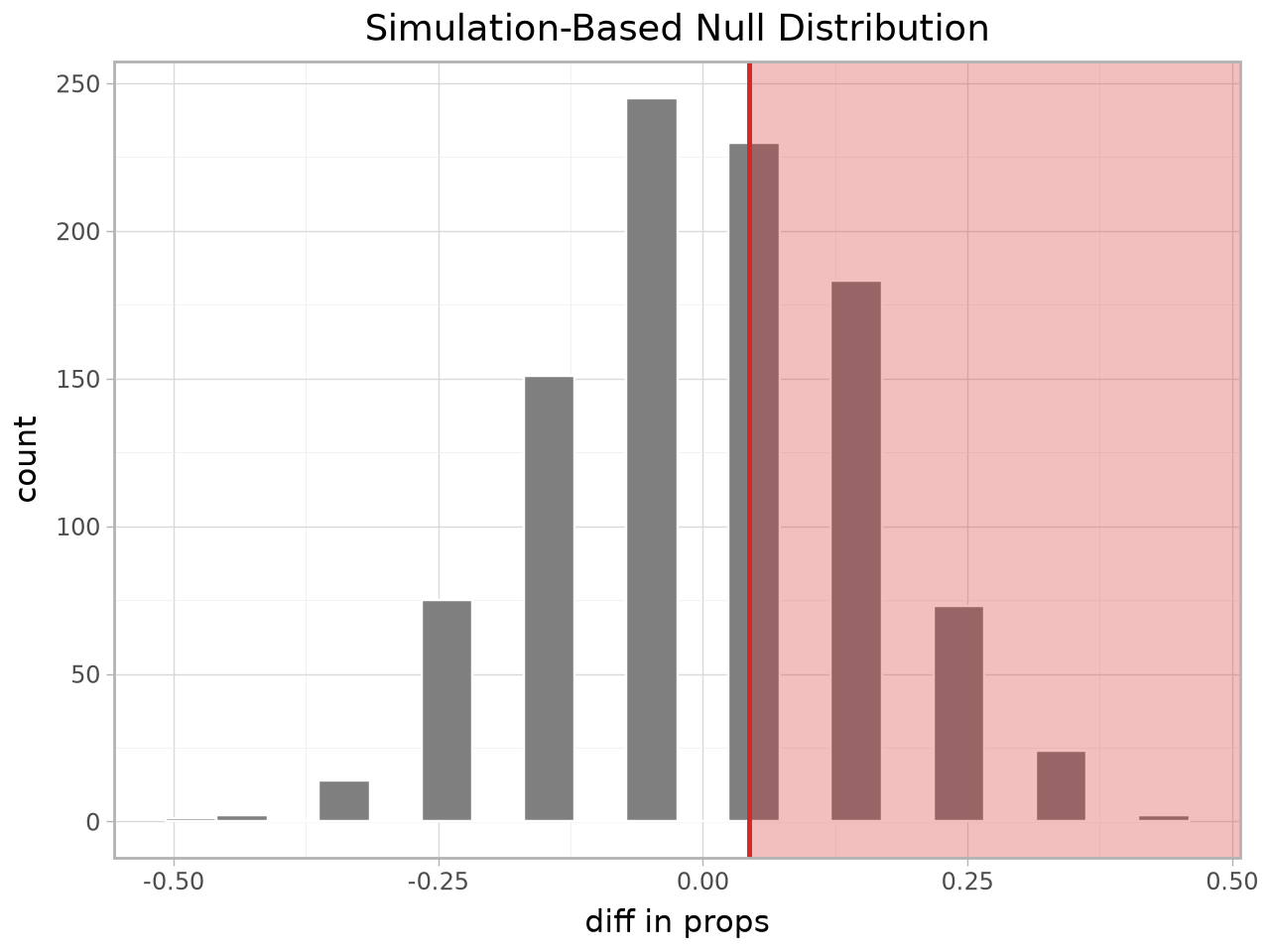
from moderndive import visualize, shade_p_value

# Interactive plotly figure
visualize(null) + shade_p_value(obs_stat=obs, direction="right")

# Same plot, plotnine
visualize(null, engine="plotnine") + shade_p_value(obs_stat=obs, direction="right")
See Plotting: plotly & plotnine for shading, confidence-interval overlays, theoretical overlays, and the regression-model plots.
Regression
import statsmodels.formula.api as smf
from moderndive import get_regression_table

houses = md.load_saratoga_houses()
model = smf.ols("price ~ living_area + bedrooms", data=houses.to_pandas()).fit()
get_regression_table(model)
| term | estimate | std_error | statistic | p_value | lower_ci | upper_ci |
|---|---|---|---|---|---|---|
| str | f64 | f64 | f64 | f64 | f64 | f64 |
| "intercept" | 20986.094 | 6816.251 | 3.079 | 0.002 | 7611.128 | 34361.06 |
| "living_area" | 93.842 | 3.109 | 30.183 | 0.0 | 87.741 | 99.943 |
| "bedrooms" | -7483.095 | 2783.531 | -2.688 | 0.007 | -12944.988 | -2021.203 |
Full details in Regression.