Regression

The regression helpers turn a fitted statsmodels model into tidy polars tables — the analog of R moderndive’s get_regression_table() / get_regression_points() / get_regression_summaries().

Fit models with statsmodels’ formula API, then tidy them:

import polars as pl
import statsmodels.formula.api as smf
import moderndive as md
from moderndive import (
    get_regression_table, get_regression_points, get_regression_summaries, get_correlation,
)

houses = md.load_saratoga_houses()
model = smf.ols("price ~ living_area + bedrooms", data=houses.to_pandas()).fit()

Coefficient table (with confidence intervals)

get_regression_table(model)

shape: (3, 7)

term	estimate	std_error	statistic	p_value	lower_ci	upper_ci
str	f64	f64	f64	f64	f64	f64
"intercept"	20986.094	6816.251	3.079	0.002	7611.128	34361.06
"living_area"	93.842	3.109	30.183	0.0	87.741	99.943
"bedrooms"	-7483.095	2783.531	-2.688	0.007	-12944.988	-2021.203

Change the confidence level with conf_level= (e.g. 0.99).

Fitted values & residuals

get_regression_points(model).head()
# columns: ID, price, living_area, bedrooms, price_hat, residual

shape: (5, 6)

ID	price	living_area	bedrooms	price_hat	residual
i64	i64	i64	i64	f64	f64
1	142212	1982	3	184531.942	-42319.942
2	134865	1676	3	155816.245	-20951.245
3	118007	1694	3	157505.404	-39498.404
4	138297	1800	2	174935.767	-36638.767
5	129470	2088	3	194479.21	-65009.21

Pass ID= to label rows by a column, and newdata= to predict on a held-out set (a residual is included when the outcome is present in newdata):

train = houses.head(800)
test = houses.tail(200)
model_train = smf.ols("price ~ living_area + bedrooms", data=train.to_pandas()).fit()
get_regression_points(model_train, newdata=test).head()

shape: (5, 6)

ID	price	living_area	bedrooms	price_hat	residual
i64	i64	i64	i64	f64	f64
1	113514	1142	2	113390.574	123.426
2	102530	1202	2	119122.741	-16592.741
3	75975	1300	3	121229.32	-45254.32
4	128434	1508	3	141100.831	-12666.831
5	185487	2271	3	213994.885	-28507.885

Model-fit summaries

get_regression_summaries(model)
# r_squared, adj_r_squared, mse, rmse, sigma, statistic (F), p_value, df, nobs

shape: (1, 9)

r_squared	adj_r_squared	mse	rmse	sigma	statistic	p_value	df	nobs
f64	f64	f64	f64	f64	f64	f64	i64	i64
0.578	0.578	2.5071e9	50071.187	50142.395	723.229	0.0	2	1057

Correlation

get_correlation(houses, "price ~ living_area")   # ≈ 0.759
# or: get_correlation(houses, x="living_area", y="price")

shape: (1, 1)

cor
f64
0.758674

Use method= for rank correlations ("spearman" or "kendall"):

get_correlation(houses, "price ~ living_area", method="spearman")

shape: (1, 1)

cor
f64
0.770381

Pass several predictors on the right-hand side to get one correlation per predictor (long by default; wide=True for one column each):

get_correlation(houses, "price ~ living_area + bedrooms + bathrooms", quiet=True)

shape: (3, 2)

predictor	cor
str	f64
"living_area"	0.758674
"bedrooms"	0.462755
"bathrooms"	0.64952

Logistic & other GLMs

The regression helpers also accept a fitted glm() model. For a logistic regression, get_regression_points() returns fitted probabilities and get_regression_summaries() returns a GLM-shaped summary (deviance, AIC, BIC, …). Pass exponentiate=True to get_regression_table() for odds ratios:

import statsmodels.api as sm

evals = md.load_evals().with_columns((pl.col("gender") == "male").cast(int).alias("is_male"))
logit = smf.glm("is_male ~ score + age", data=evals.to_pandas(),
                family=sm.families.Binomial()).fit()
get_regression_table(logit, exponentiate=True)

shape: (3, 7)

term	estimate	std_error	statistic	p_value	lower_ci	upper_ci
str	f64	f64	f64	f64	f64	f64
"intercept"	0.003	1.029	-5.611	0.0	0.0	0.023
"score"	1.954	0.188	3.561	0.0	1.351	2.825
"age"	1.071	0.011	6.292	0.0	1.049	1.095

get_regression_summaries(logit)

shape: (1, 10)

mse	rmse	deviance	null_deviance	aic	bic	log_lik	df_residual	df_null	nobs
f64	f64	f64	f64	f64	f64	f64	i64	i64	i64
0.219	0.468	578.298	630.296	584.298	596.711	-289.149	460	462	463

Array-API models

You don’t have to use the formula API. The helpers also accept models fit with statsmodels’ array API (sm.OLS(y, X) / sm.GLM(...)), which is handy when your design matrix is already built. get_regression_points() reconstructs the per-observation table from the design matrix (the constant column becomes the intercept term and is dropped from the points):

import statsmodels.api as sm

X = sm.add_constant(houses.select("living_area", "bedrooms").to_pandas())
y = houses["price"].to_pandas()
array_model = sm.OLS(y, X).fit()

get_regression_table(array_model)

shape: (3, 7)

term	estimate	std_error	statistic	p_value	lower_ci	upper_ci
str	f64	f64	f64	f64	f64	f64
"intercept"	20986.094	6816.251	3.079	0.002	7611.128	34361.06
"living_area"	93.842	3.109	30.183	0.0	87.741	99.943
"bedrooms"	-7483.095	2783.531	-2.688	0.007	-12944.988	-2021.203

get_regression_points(array_model).head()

shape: (5, 6)

ID	price	living_area	bedrooms	price_hat	residual
i64	f64	f64	f64	f64	f64
1	142212.0	1982.0	3.0	184531.942	-42319.942
2	134865.0	1676.0	3.0	155816.245	-20951.245
3	118007.0	1694.0	3.0	157505.404	-39498.404
4	138297.0	1800.0	2.0	174935.767	-36638.767
5	129470.0	2088.0	3.0	194479.21	-65009.21

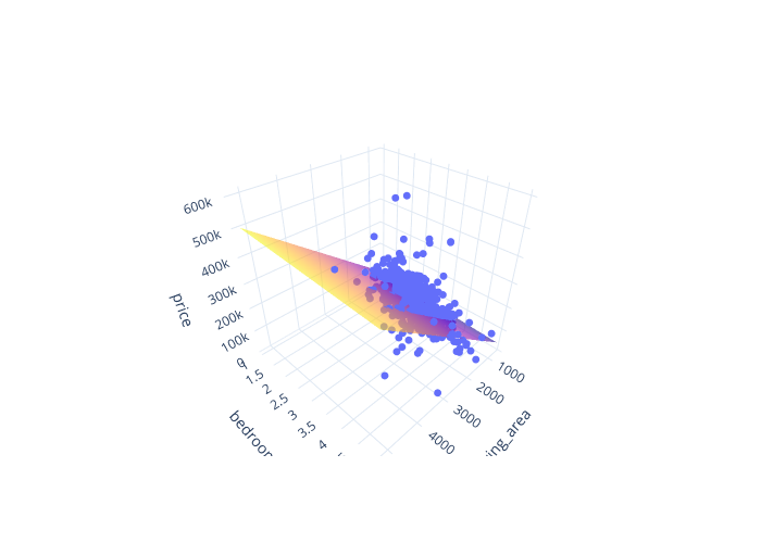
3D regression plane

plot_3d_regression() draws an interactive 3D scatter of an outcome against two numeric predictors, with the fitted regression plane overlaid (a plotly figure):

from moderndive import plot_3d_regression

plot_3d_regression(houses, "price ~ living_area + bedrooms")

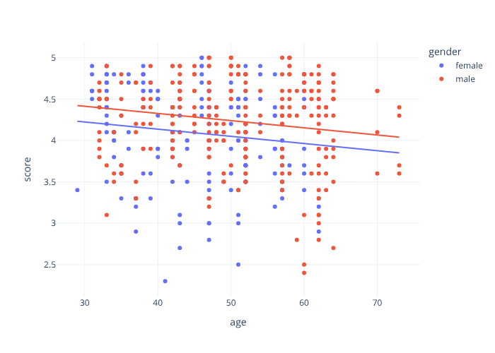
Visualizing models

Two ports of R moderndive’s ggplot helpers, both dual-engine. A parallel-slopes model — one common slope with a separate intercept per group:

from moderndive import gg_parallel_slopes, gg_categorical_model

evals = md.load_evals()
gg_parallel_slopes(evals, response="score", explanatory="age", by="gender")  # plotly

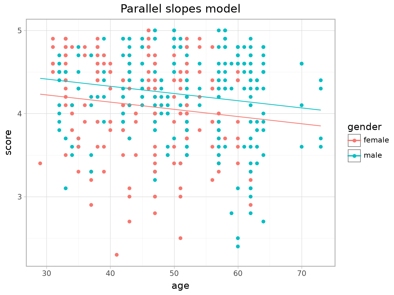
The same plot via the plotnine engine:

gg_parallel_slopes(evals, response="score", explanatory="age", by="gender", engine="plotnine")

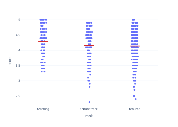
A regression with a single categorical predictor (geom_categorical_model() is an alias of gg_categorical_model()):

gg_categorical_model(evals, response="score", explanatory="rank")

For the plotnine engine you can also drop the parallel-slopes lines onto your own ggplot with geom_parallel_slopes().

Inference for regression coefficients

fit() runs the regression on every bootstrap/permutation replicate, giving a distribution per coefficient. Pair it with visualize_fit and per-facet shading:

from moderndive import specify
from moderndive.infer.viz import visualize_fit
from moderndive import shade_confidence_interval, shade_p_value

f = "price ~ living_area + bedrooms"
obs_fit = houses.specify(formula=f).fit()

# Bootstrap distribution of each coefficient → per-term CIs
boot_fit = houses.specify(formula=f).generate(reps=1000, type="bootstrap", seed=1).fit()
boot_fit.get_confidence_interval(level=0.95)          # one row per term
visualize_fit(boot_fit) + shade_confidence_interval(boot_fit.get_confidence_interval())

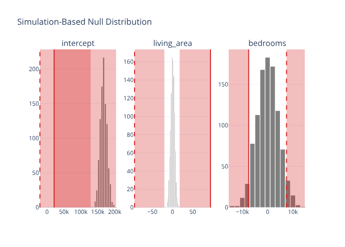
# Null distribution → per-term p-values, each facet shaded at its own estimate
null_fit = (
    houses.specify(formula=f).hypothesize(null="independence")
    .generate(reps=1000, type="permute", seed=1).fit()
)
null_fit.get_p_value(obs_stat=obs_fit, direction="two-sided")
visualize_fit(null_fit) + shade_p_value(obs_stat=obs_fit, direction="two-sided")

Per-facet shading works in both engines: shade_p_value / shade_confidence_interval accept the observed FitResult or a term-keyed table, and each facet is shaded from its own value.