Pipeline examples (the infer “stat menu”)¶

This page follows the R infer observed-statistic examples vignette: the calculate(stat=...) forms organized by the types of variables involved, using the same gss dataset (a sample from the US General Social Survey) that ships with the package.

import moderndive as md
from moderndive import get_p_value, get_confidence_interval, assume

gss = md.load_gss()
gss.head()

shape: (5, 11)

year	age	sex	college	partyid	hompop	hours	income	class	finrela	weight
i64	i64	str	str	str	i64	i64	str	str	str	f64
2014	36	"male"	"degree"	"ind"	3	50	"$25000 or more"	"middle class"	"below average"	0.896003
1994	34	"female"	"no degree"	"rep"	4	31	"$20000 - 24999"	"working class"	"below average"	1.0825
1998	24	"male"	"degree"	"ind"	1	40	"$25000 or more"	"working class"	"below average"	0.5501
1996	42	"male"	"no degree"	"ind"	4	40	"$25000 or more"	"working class"	"above average"	1.0864
1994	31	"male"	"degree"	"rep"	2	40	"$25000 or more"	"middle class"	"above average"	1.0825

Throughout, the pattern is the same as in R infer:

the observed statistic comes from specify() → [hypothesize()] → calculate();
a null distribution comes from adding generate() before calculate();
a bootstrap distribution (for confidence intervals) comes from generate(type="bootstrap") with no hypothesize().

One numerical variable¶

# mean
gss.specify(response="hours").calculate(stat="mean")

ObservedStatistic(stat='mean', value=41.382)

# median, then standard deviation
print(gss.specify(response="hours").calculate(stat="median"))
print(gss.specify(response="hours").calculate(stat="sd"))

ObservedStatistic(stat='median', value=40)
ObservedStatistic(stat='sd', value=14.82)

Standardized mean (one-sample t) — needs a hypothesized mu:

gss.specify(response="hours").hypothesize(null="point", mu=40).calculate(stat="t")

ObservedStatistic(stat='t', value=2.08519)

A full one-mean test — null distribution and p-value:

obs_mean = gss.specify(response="hours").calculate(stat="mean")
null_mean = (
    gss.specify(response="hours")
    .hypothesize(null="point", mu=40)
    .generate(reps=1000, type="bootstrap", seed=1)
    .calculate(stat="mean")
)
get_p_value(null_mean, obs_stat=obs_mean, direction="two-sided")

shape: (1, 1)

p_value
f64
0.03

…and a bootstrap confidence interval for the mean:

boot_mean = (
    gss.specify(response="hours")
    .generate(reps=1000, type="bootstrap", seed=1)
    .calculate(stat="mean")
)
get_confidence_interval(boot_mean, level=0.95, type="percentile")

shape: (1, 2)

lower_ci	upper_ci
f64	f64
40.12395	42.608

One categorical variable¶

# proportion of a "success" level, then the raw count
print(gss.specify(response="sex", success="female").calculate(stat="prop"))
print(gss.specify(response="sex", success="female").calculate(stat="count"))

ObservedStatistic(stat='prop', value=0.474)
ObservedStatistic(stat='count', value=237)

Standardized proportion (one-sample z) — needs a hypothesized p:

gss.specify(response="sex", success="female").hypothesize(null="point", p=0.5).calculate(stat="z")

ObservedStatistic(stat='z', value=-1.16276)

A one-proportion test by simulation (draw, alias simulate):

obs_prop = gss.specify(response="sex", success="female").calculate(stat="prop")
null_prop = (
    gss.specify(response="sex", success="female")
    .hypothesize(null="point", p=0.5)
    .generate(reps=1000, type="draw", seed=1)
    .calculate(stat="prop")
)
get_p_value(null_prop, obs_stat=obs_prop, direction="two-sided")

shape: (1, 1)

p_value
f64
0.286

One categorical variable (3+ levels): chi-square goodness-of-fit¶

Test whether the counts across a variable’s levels match a set of hypothesized proportions. Pass p as a {level: probability} mapping to hypothesize(null="point", ...), then generate(type="draw") to simulate from those proportions:

levels = gss["finrela"].unique().to_list()
uniform = {level: 1 / len(levels) for level in levels}  # "all classes equally likely"

obs_gof = gss.specify(response="finrela").hypothesize(null="point", p=uniform).calculate(stat="Chisq")
null_gof = (
    gss.specify(response="finrela")
    .hypothesize(null="point", p=uniform)
    .generate(reps=1000, type="draw", seed=1)
    .calculate(stat="Chisq")
)
get_p_value(null_gof, obs_stat=obs_gof, direction="greater")

shape: (1, 1)

p_value
f64
0.0

The one-line wrapper is chisq_test(gss, response="finrela", p=uniform).

Two categorical variables (2 levels each)¶

# difference in proportions of "degree" between the sexes
gss.specify(formula="college ~ sex", success="degree").calculate(
    stat="diff in props", order=("male", "female")
)

ObservedStatistic(stat='diff in props', value=-0.00420337)

# ratio of proportions and the odds ratio
spec = gss.specify(formula="college ~ sex", success="degree")
print(spec.calculate(stat="ratio of props", order=("male", "female")))
print(spec.calculate(stat="odds ratio", order=("male", "female")))

ObservedStatistic(stat='ratio of props', value=0.987998)
ObservedStatistic(stat='odds ratio', value=0.981648)

Standardized difference in proportions (z):

gss.specify(formula="college ~ sex", success="degree").calculate(
    stat="z", order=("male", "female")
)

ObservedStatistic(stat='z', value=-0.098526)

Two categorical variables (chi-square test of independence)¶

obs_chisq = gss.specify(formula="finrela ~ sex").calculate(stat="Chisq")
obs_chisq

ObservedStatistic(stat='Chisq', value=9.1054)

null_chisq = (
    gss.specify(formula="finrela ~ sex")
    .hypothesize(null="independence")
    .generate(reps=1000, type="permute", seed=1)
    .calculate(stat="Chisq")
)
get_p_value(null_chisq, obs_stat=obs_chisq, direction="greater")

shape: (1, 1)

p_value
f64
0.1

A chi-square test is inherently one-sided; the theoretical distribution agrees:

n_levels_finrela = gss["finrela"].n_unique()
df_chisq = (n_levels_finrela - 1) * (gss["sex"].n_unique() - 1)
assume("Chisq", df=df_chisq).get_p_value(obs_chisq, direction="greater")

shape: (1, 1)

p_value
f64
0.104933

One numerical and one categorical variable (2 levels)¶

# difference in mean age by college degree
gss.specify(formula="age ~ college").calculate(
    stat="diff in means", order=("degree", "no degree")
)

ObservedStatistic(stat='diff in means', value=0.94066)

# difference in medians, ratio of means, and the two-sample t
spec = gss.specify(formula="age ~ college")
print(spec.calculate(stat="diff in medians", order=("degree", "no degree")))
print(spec.calculate(stat="ratio of means", order=("degree", "no degree")))
print(spec.calculate(stat="t", order=("degree", "no degree")))

ObservedStatistic(stat='diff in medians', value=3)
ObservedStatistic(stat='ratio of means', value=1.02355)
ObservedStatistic(stat='t', value=0.802379)

Null distribution and p-value for the difference in means:

obs_diff = gss.specify(formula="age ~ college").calculate(
    stat="diff in means", order=("degree", "no degree")
)
null_diff = (
    gss.specify(formula="age ~ college")
    .hypothesize(null="independence")
    .generate(reps=1000, type="permute", seed=1)
    .calculate(stat="diff in means", order=("degree", "no degree"))
)
get_p_value(null_diff, obs_stat=obs_diff, direction="two-sided")

shape: (1, 1)

p_value
f64
0.44

One numerical and one categorical variable (3+ levels): ANOVA F¶

gss.specify(formula="age ~ partyid").calculate(stat="F")

ObservedStatistic(stat='F', value=2.48421)

Two numerical variables¶

# Pearson correlation, then the regression slope
print(gss.specify(formula="hours ~ age").calculate(stat="correlation"))
print(gss.specify(formula="hours ~ age").calculate(stat="slope"))

ObservedStatistic(stat='correlation', value=0.00701719)
ObservedStatistic(stat='slope', value=0.00780766)

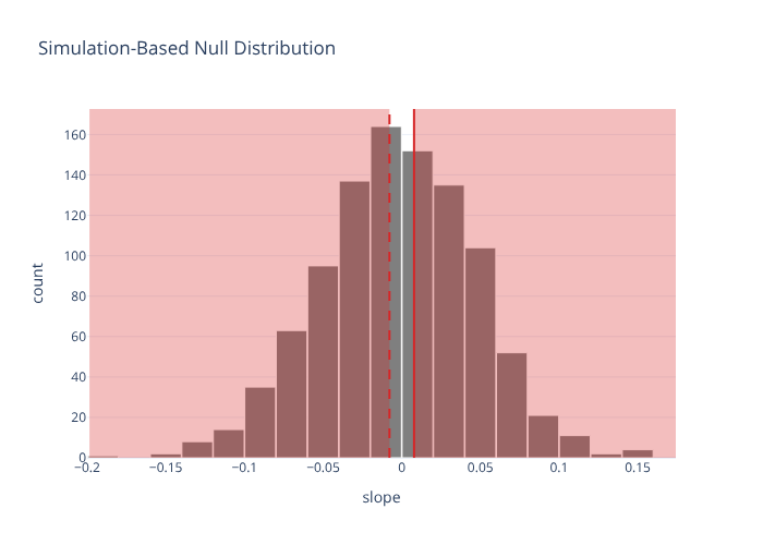
A permutation test for the slope, visualized:

from moderndive import visualize, shade_p_value

obs_slope = gss.specify(formula="hours ~ age").calculate(stat="slope")
null_slope = (
    gss.specify(formula="hours ~ age")
    .hypothesize(null="independence")
    .generate(reps=1000, type="permute", seed=1)
    .calculate(stat="slope")
)
visualize(null_slope) + shade_p_value(obs_stat=obs_slope, direction="two-sided")

../_images/2cc01866a0a345972994b48ee6f7c2e2a7ae4cc6817b599161c0185da32a4e30.png

Custom statistics¶

Any of the above can be swapped for a callable returning a single number — see the custom-statistic example in Hypothesis testing.